![]() GEARS - Geospatial Ecology and Remote Sensing lab - https://www.geospatialecology.com
GEARS - Geospatial Ecology and Remote Sensing lab - https://www.geospatialecology.com
Introduction to Remote Sensing of the Environment
Lab 10 - Working with Terrestrial Laser Scanning (TLS) data in CloudCompare continued
Prerequisites
Completion of this lab exercise requires use of the CloudCompare software package. CloudCompare is a powerful package for visualising and processing point-clouds, and best of all is open-access. You can download the version to match your operating system here:
https://www.danielgm.net/cc/
Background and objective
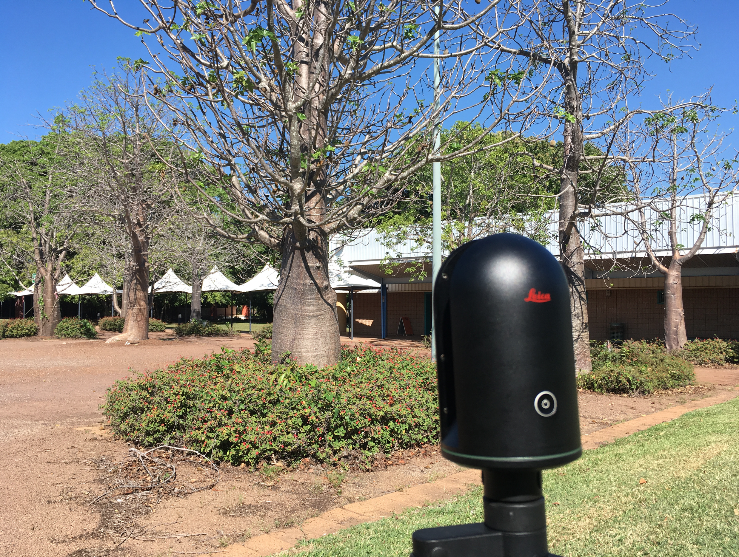
The objective of this lab is to familiarise yourself with 3D point cloud data. We will use data that we collected last week on campus in the Boab court. We collected multiple scans with a Leica BLK360 laser scanner, and we will work with some of these scans today.
Scan data can be downloaded in .las format here (please note that each file is ~ 1GB):
Getting to know CloudCompare
Please see Lab 9 from my "Introduction to Remote Sensing" before continuing.
Merging multiple point clouds
-
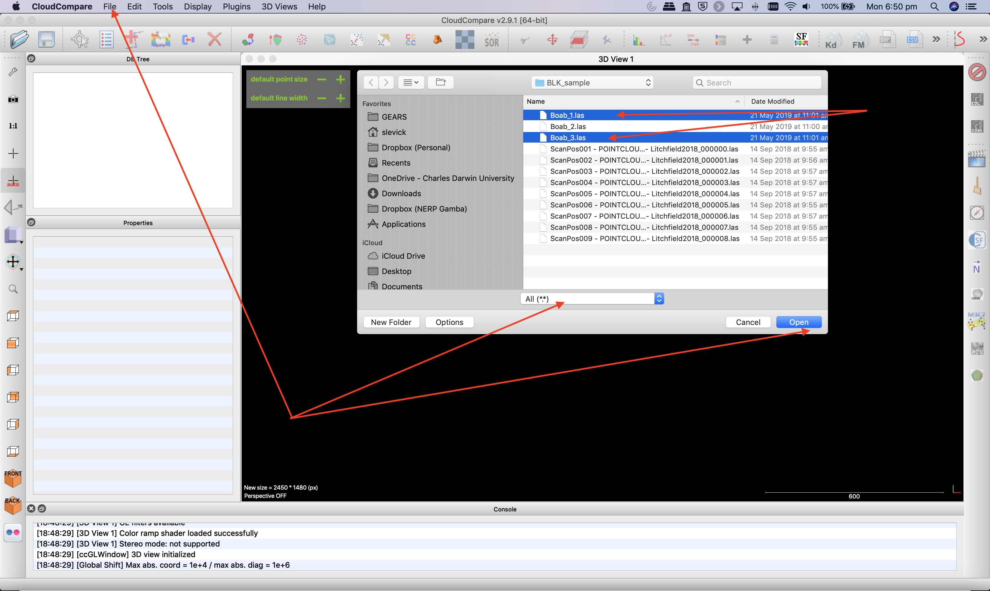
Open up CloudCompare and choose File>Open from the main menu.
-
Navigate to where the scan data are stored and select Boab_1.las and Boab_3.las before clicking "Open". If you cannot see your files or they are greyed out, make sure you have the file type set to ".las" or "All".
-
Click "Apply to all" and "Yes to all" when the two dialogue boxes pop up.
-
Once the two files have loaded, you will see that they are not correctly aligned.
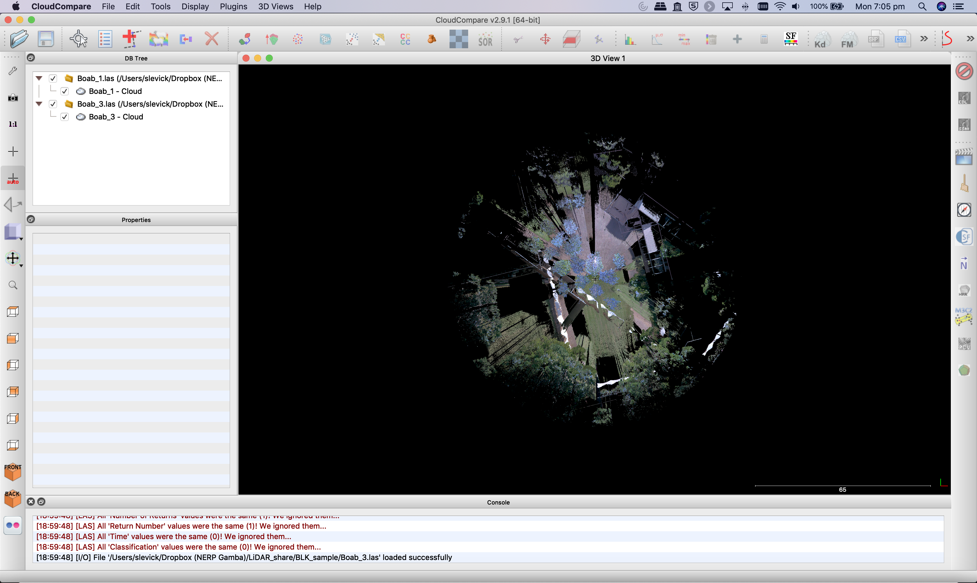
- In fact, if you zoom in closer (using the mouse wheel), you will see that they are positioned exactly on top of each other (even though they were collected ~ 10m apart).
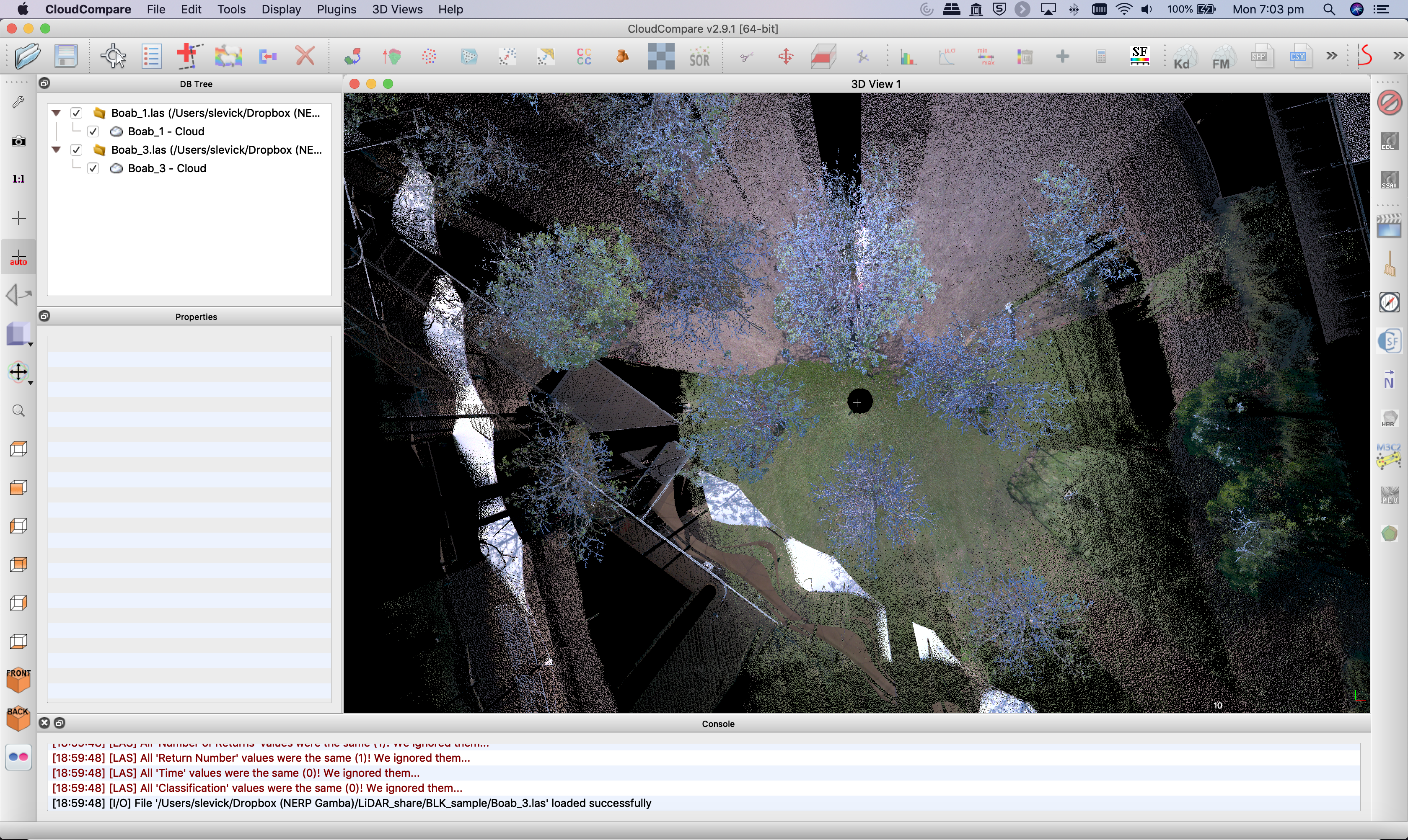
-
This issues occurs because the scans are in the scanners own coordinated system (SOC) and not in a geographic coordinate system (the BLK360 lacks a GPS). The origin of both scans is 0,0,0 (x,y,z) - every point is relative to the scanner itself.
-
We will align these two scans using a combination of manual translation (rough positioning) and an automated computer algorithm called Iterative Closest Point (ICP) for fine tuning.
-
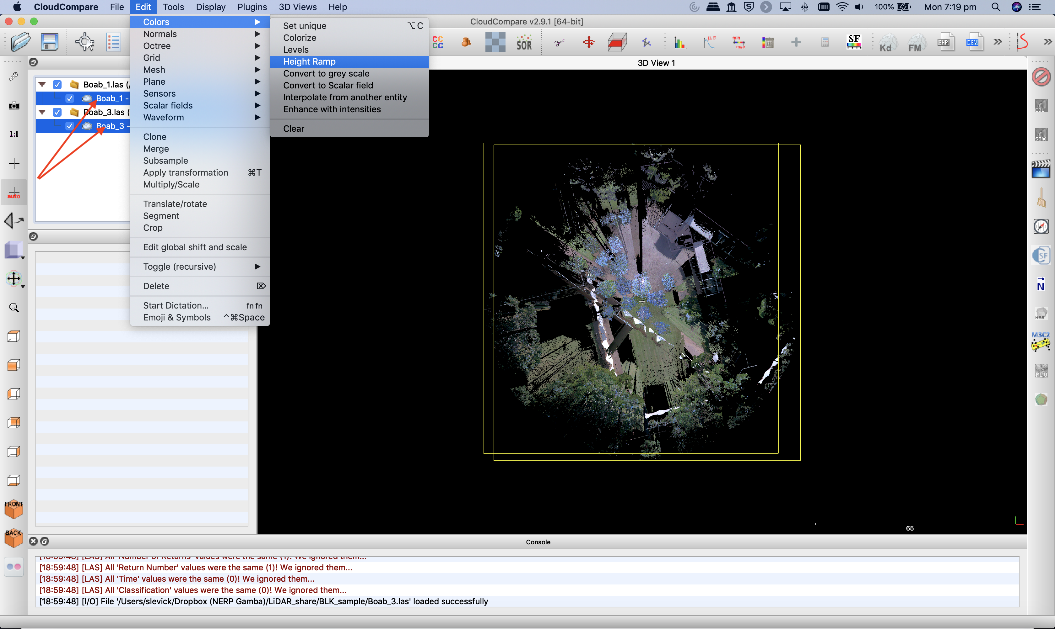
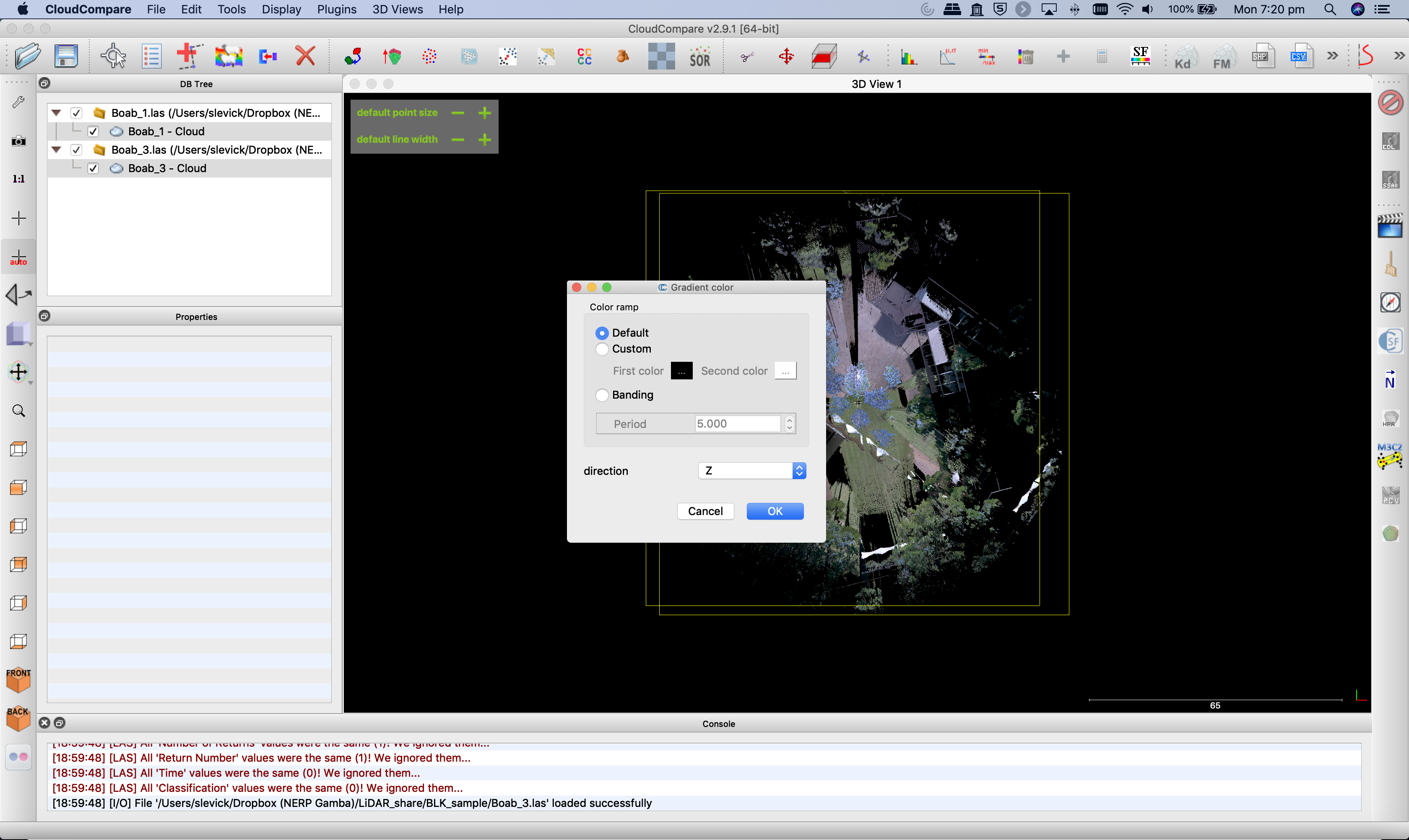
Before starting with this, let us map both clouds according to an elevation colour scale (height ramp) - using the default scale for blue to green. Be sure to select both clouds before applying the colour ramp.
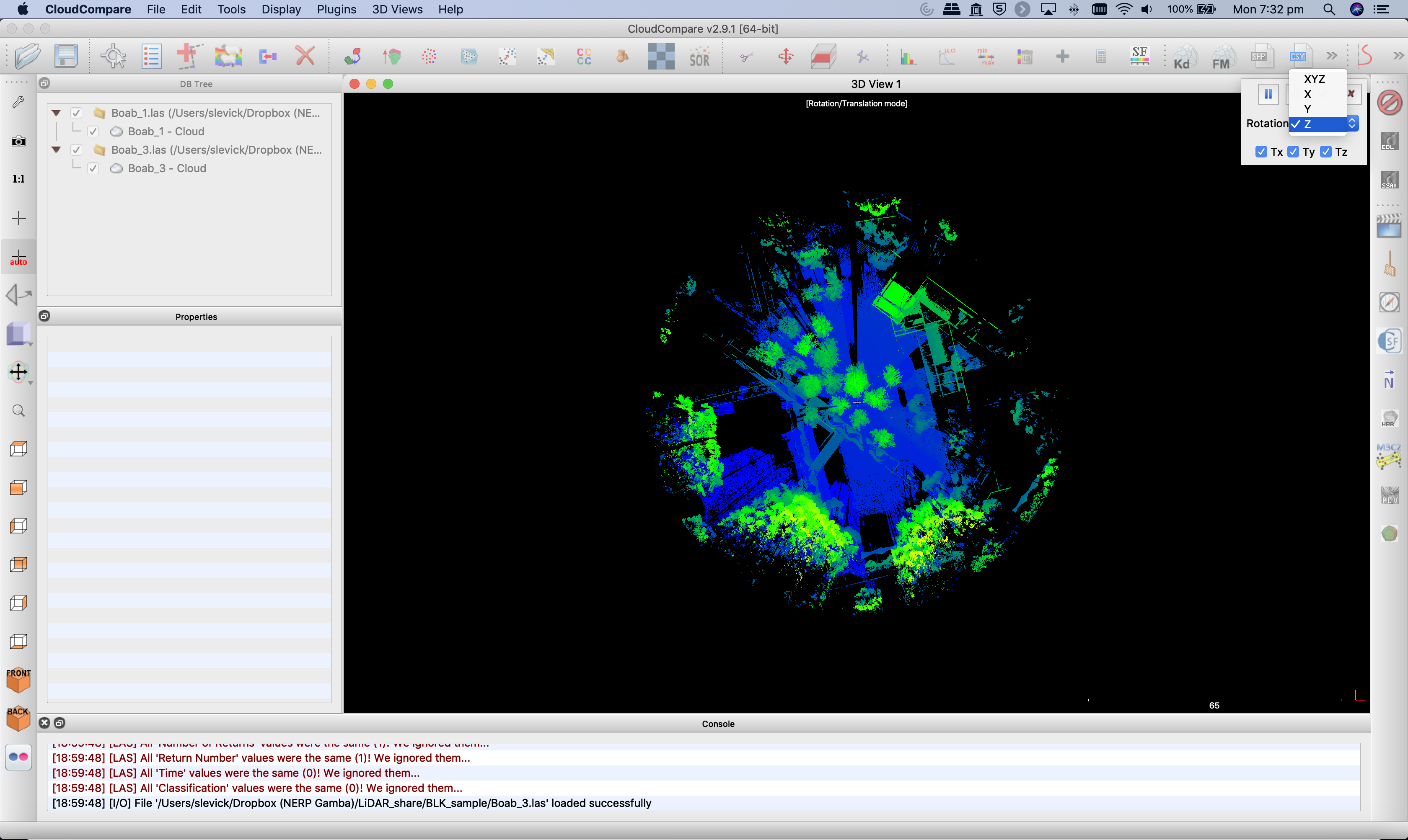
- Next select only the Boab_3.las file, and choose the "Translate" tool from either the main Menu or from the icon in the toolbar.
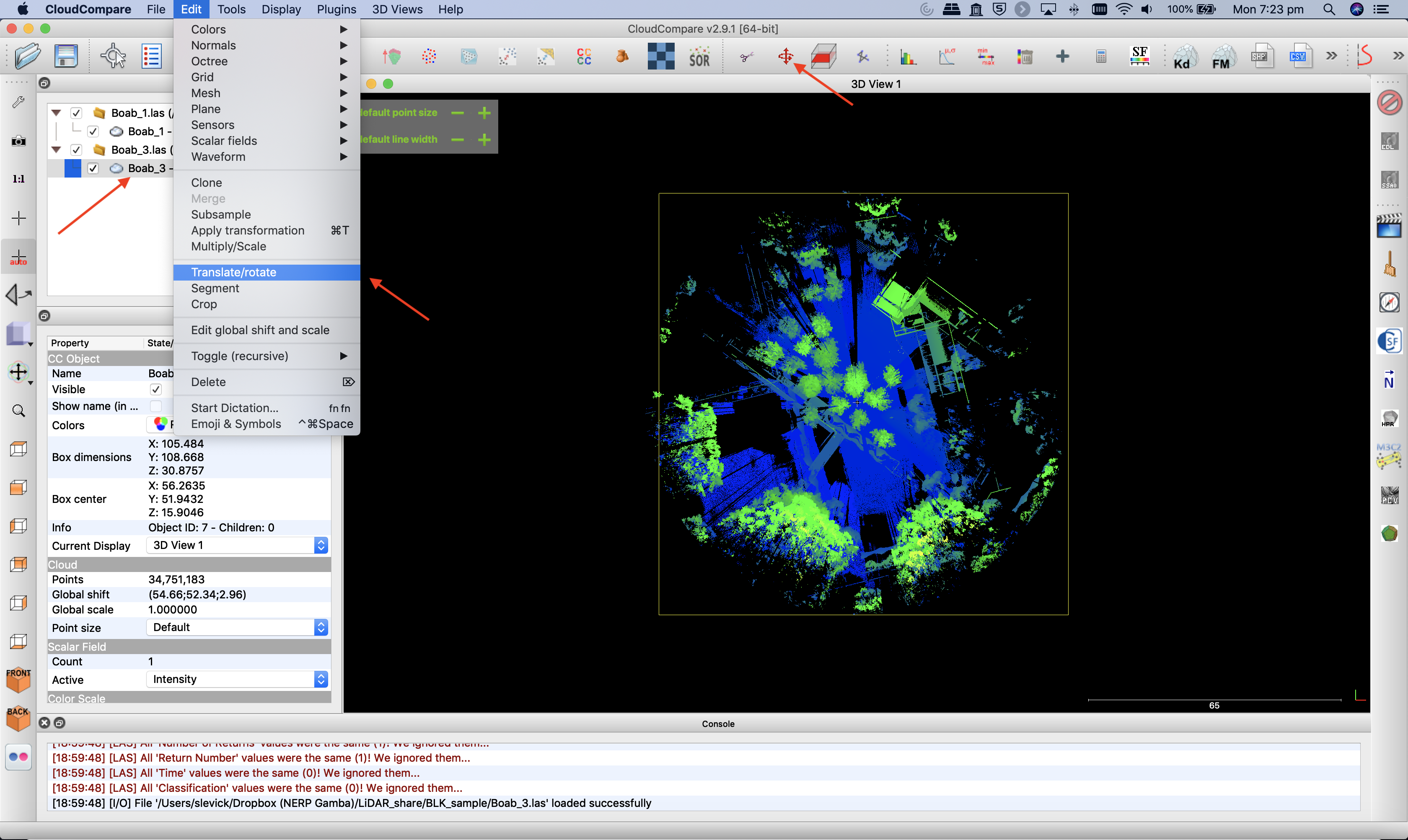
- You will see a new toolbar appear in the top-right corner of the main window, and small white text in the top-centre of the main window will remind you that the tool is active.
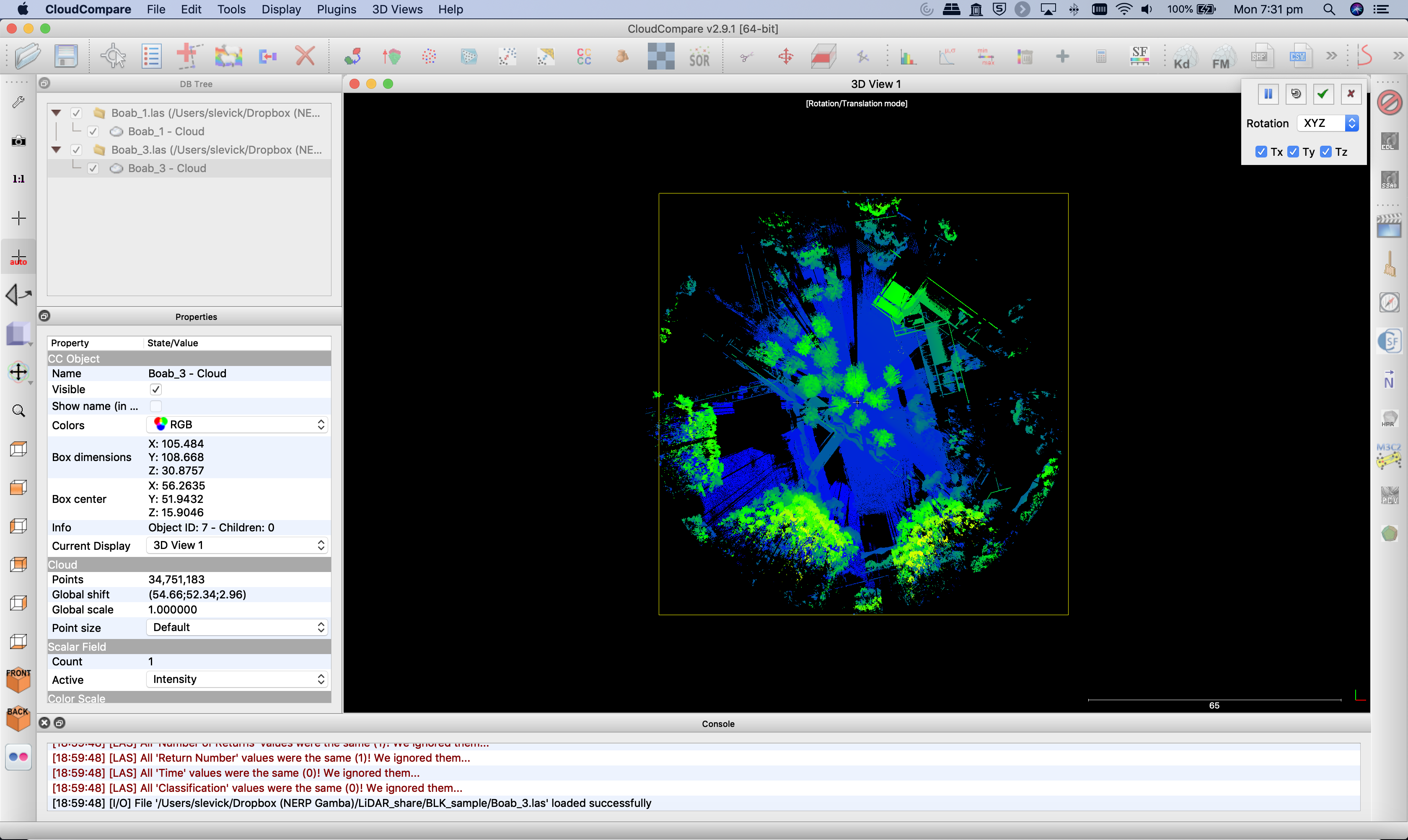
- Before going any further we will change the rotation axis from xyz to z only in the translation dialogue window. This will ensure that the point cloud can only be moved (left/right, up/down) or rotated around the z x-axis, preventing any unwanted tilting.
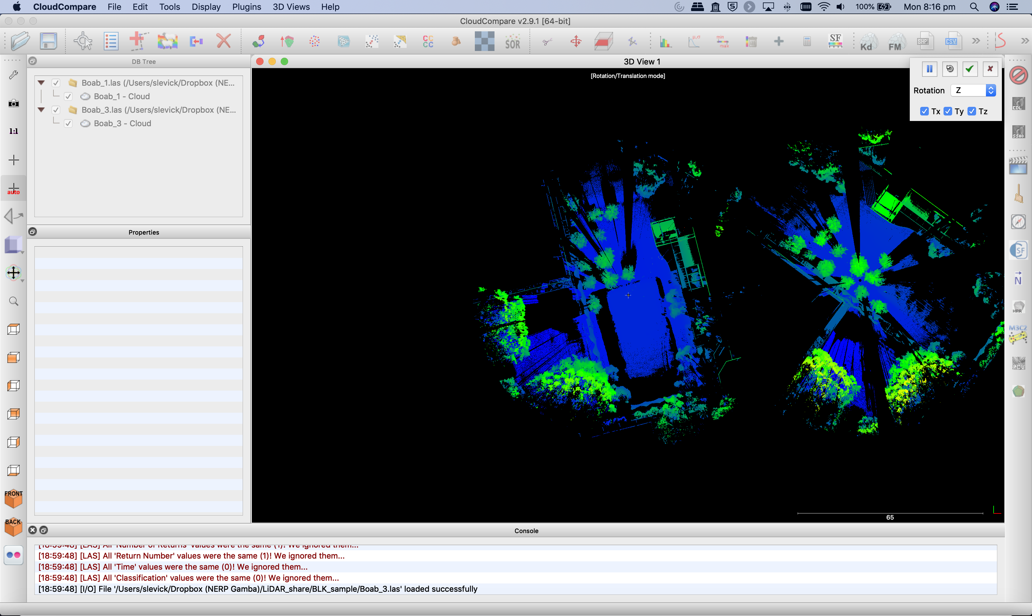
- Now we can use the right-mouse click to drag the selected cloud (Boab_3) in any direction we like - in the screenshot below you will see I have shifted it over to the right.
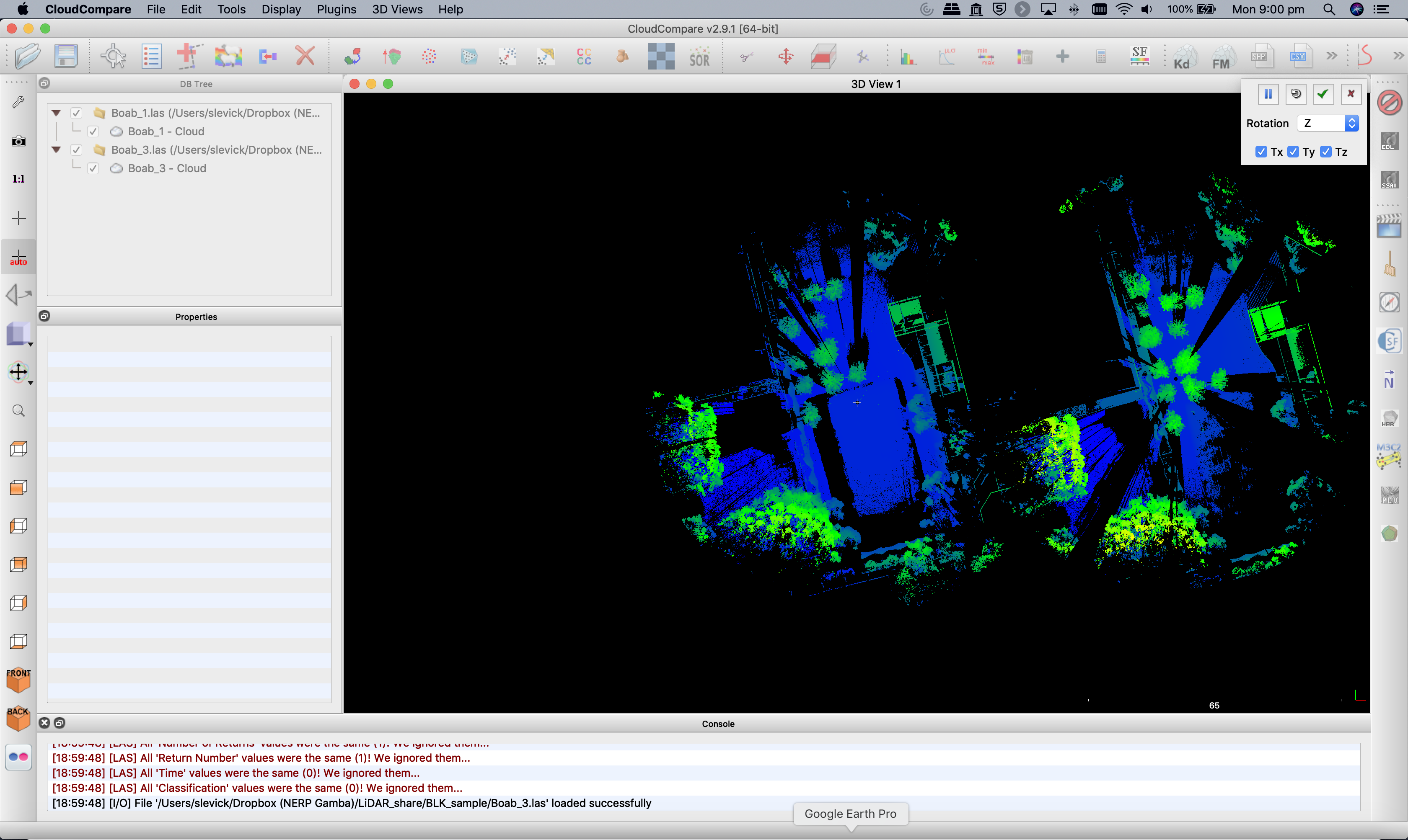
- Now we can see the two scans clearly, and we can see that Boab_3 needs to be rotated clockwise to align better with Boab_1. Using the left mouse button click and drag the Boab_3 cloud to rotate it by about 30 degrees in teh clockwise direction.
-
Now that the rotation looks better, we can use the right-mouse button to pull the whole cloud over to the left again and position it in better alignment with Boab_1.
-
That looks much better, so now we can click the green tick to accept these changes to the orientation matrix of Boab_3.
-
If we zoom in, we can now see the two separate scan locations, they are no longer on top of each other but are very nearly in the correct position.
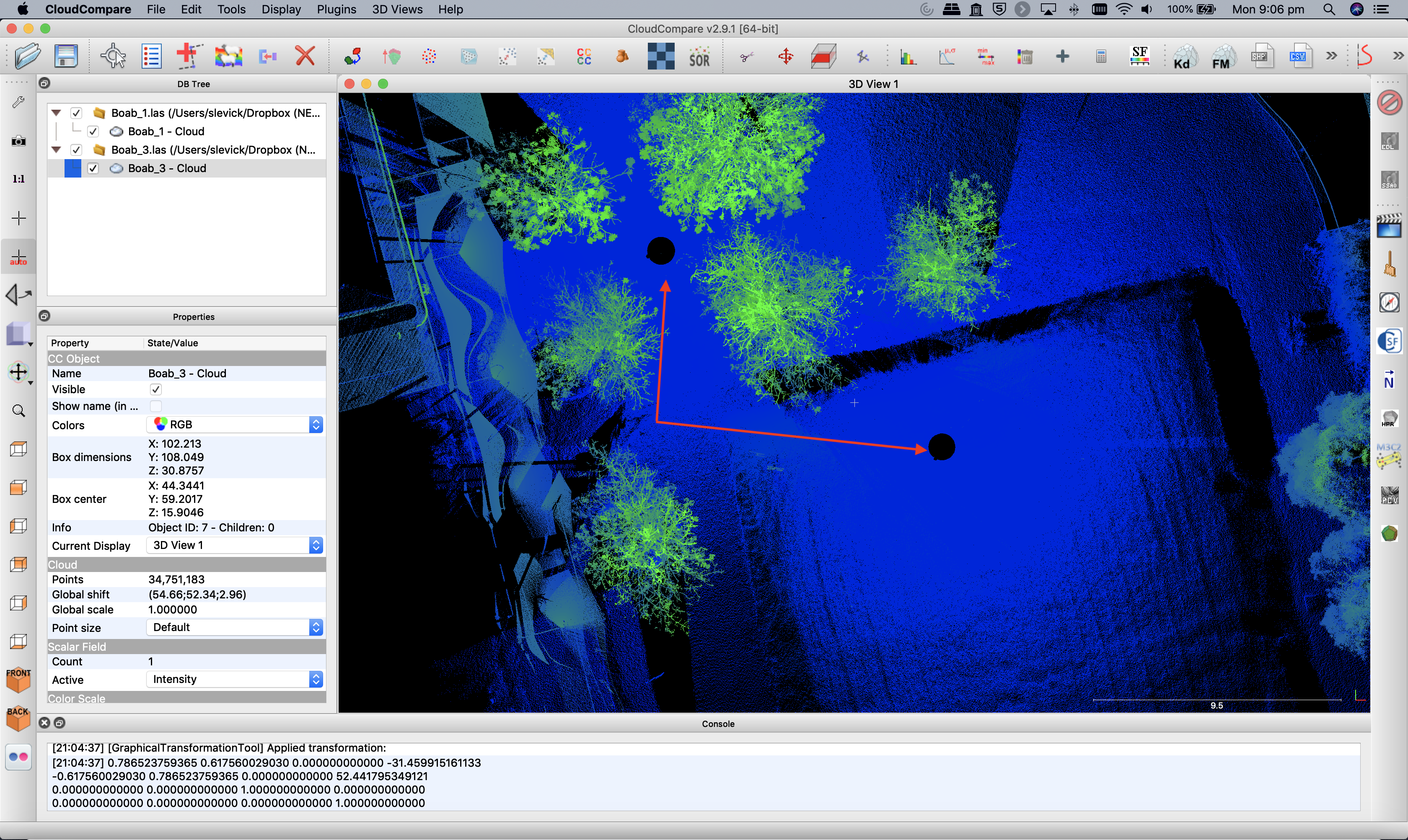
- However if we examine some straight lines for example, it is still clear that some minor offset is present.

- We will correct this in Part 3 using the ICP algorithm
Thank you
I hope you found that useful. A recorded video of this tutorial can be found on my YouTube Channel's Introduction to Remote Sensing of the Environment Playlist and on my lab website GEARS.